9.2. Isotopically Non-Stationary 13C-MFA
INCA is capable of analyzing isotopically non-stationary (INST) data. I such data sets the fluxes are still assumed to be constant, however the isotopologue distribution vector are allow to vary dynamically (See plot further down).
The INCAWrapper can setup INCA models to fit INST datasets. In this example we will show how by estimating the flux distribution from a simulated INST dataset.
The simulated dataset is produced using the simple model [1,2], which we have also used in earlier tutorials. This time however, we simulated the isotopically non-stationary data. To inspect how the data was simulated see https://github.com/biosustain/incawrapper/tree/main/docs/examples/Literature%20data/simple%20model/simple_model_inst_simulation.py.
[1]:
import pandas as pd
import pathlib
import incawrapper
import ast
PROJECT_DIR = pathlib.Path().cwd().parents[1].resolve()
data_folder = PROJECT_DIR / pathlib.Path("docs/examples/Literature data/simple model")
To fit fluxes to a INST dataset INCA as minimum requires:
Reaction data
Tracer data
MS measurements
Furthermore, it is possible to use - Flux measurements - Pool size measurement, i.e. concentrations of metabolites
For completeness, we will here consider the data where we have ms, pool size, and flux measurements. We will load both the measurements and the tracer and reaction information here.
[2]:
tracers_data = pd.read_csv(data_folder / "tracers.csv",
   converters={'atom_mdv':ast.literal_eval, 'atom_ids':ast.literal_eval} # a trick to read lists from csv
).query("experiment_id == 'exp1'") # we only simulated experiment 1

reactions_data = pd.read_csv(data_folder / "reactions.csv")
ms_data = pd.read_csv(data_folder / 'simulated_data' / "mdv_no_noise.csv",
   converters={'labelled_atom_ids': ast.literal_eval} # a trick to read lists from csv
)
pool_sizes = pd.read_csv(data_folder / 'simulated_data' / "pool_sizes_measurement_no_noise.csv")
flux_measurements = pd.read_csv(data_folder / 'simulated_data' / "flux_measurements_no_noise.csv")
The toy model has 5 reactions that we will show here.
[3]:
reactions_data.head()
[3]:
| model | rxn_id | rxn_eqn | |
|---|---|---|---|
| 0 | simple_model | R1 | A (abc) -> B (abc) |
| 1 | simple_model | R2 | B (abc) <-> D (abc) |
| 2 | simple_model | R3 | B (abc) -> C (bc) + E (a) |
| 3 | simple_model | R4 | B (abc) + C (de) -> D (bcd) + E (a) + E (e) |
| 4 | simple_model | R5 | D (abc) -> F (abc) |
We consider one experiment with a single labelled substrate, A, which is labelled at carbon position 2.
[4]:
tracers_data.head()
[4]:
| experiment_id | met_id | tracer_id | atom_ids | ratio | atom_mdv | enrichment | |
|---|---|---|---|---|---|---|---|
| 0 | exp1 | A | [2-13C]A | [2] | 1.0 | [0, 1] | 1 |
When analysing INST data, we have mass distribution vectors of the same metabolite at multiple time points. These are specified by adding the timepoint in the time column.
[5]:
ms_data.head()
[5]:
| experiment_id | met_id | ms_id | measurement_replicate | labelled_atom_ids | unlabelled_atoms | mass_isotope | intensity_std_error | time | intensity | |
|---|---|---|---|---|---|---|---|---|---|---|
| 0 | exp1 | B | B1 | 1 | [1, 2, 3] | NaN | 0 | 0.003 | 0 | 1.0 |
| 1 | exp1 | B | B1 | 1 | [1, 2, 3] | NaN | 1 | 0.003 | 0 | 0.0 |
| 2 | exp1 | B | B1 | 1 | [1, 2, 3] | NaN | 2 | 0.003 | 0 | 0.0 |
| 3 | exp1 | B | B1 | 1 | [1, 2, 3] | NaN | 3 | 0.003 | 0 | 0.0 |
| 4 | exp1 | F | F1 | 1 | [1, 2, 3] | NaN | 0 | 0.003 | 0 | 1.0 |
To get a better idea of what the data looks like we can visualise the time series.
[6]:
import seaborn as sns
import matplotlib.pyplot as plt

g = sns.FacetGrid(ms_data, col="ms_id", hue="mass_isotope")
g.map_dataframe(sns.lineplot, data=ms_data, x="time", y="intensity")

# add overall legend
g.add_legend()
/Users/s143838/.virtualenvs/incawrapper-dev/lib/python3.10/site-packages/seaborn/axisgrid.py:123: UserWarning: The figure layout has changed to tight
  self._figure.tight_layout(*args, **kwargs)
[6]:
<seaborn.axisgrid.FacetGrid at 0x123ee1630>
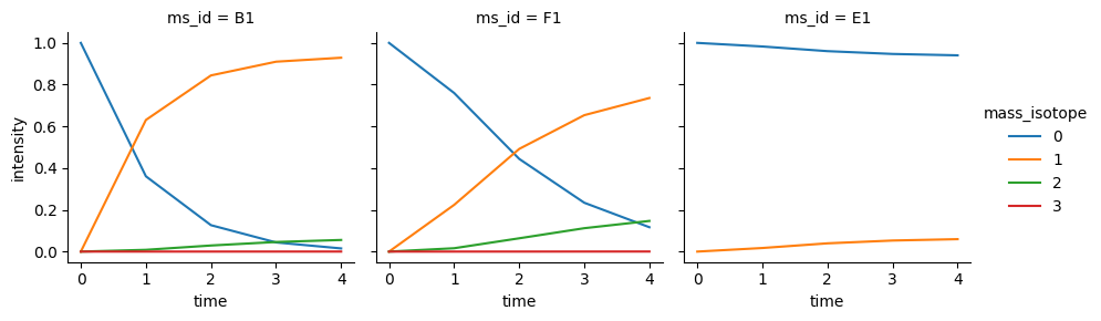
We see that the measured mass isotopologue distribution changes over time especially for the B and F metabolites. While it only changes a little for the E metabolite.
We also have measurements of one uptake rate and one secretion rate. A core assumption for INST 13C-MFA is that the fluxes are constant, thus there is only one measurement for each flux.
[7]:
flux_measurements.head()
[7]:
| rxn_id | flux | experiment_id | flux_std_error | |
|---|---|---|---|---|
| 0 | R1 | 100.000000 | exp1 | 0.300000 |
| 1 | R5 | 80.566147 | exp1 | 0.241698 |
Now, we are ready to create the inca script. This is done very similar to the other examples. The main difference is that sim_ss=False this tells inca that don’t wish to assume steady state in the isotopologue distributions.
[8]:
output_file = PROJECT_DIR / pathlib.Path("docs/examples/Literature data/simple model/simple_model_inst_fitting.mat")
script = incawrapper.create_inca_script_from_data(
    reactions_data=reactions_data,
    tracer_data=tracers_data,
    flux_measurements=flux_measurements,
    pool_measurements=pool_sizes,
    ms_measurements=ms_data,
    experiment_ids=["exp1"]
)
script.add_to_block("options",
    incawrapper.define_options(
        fit_starts=10, # Number of flux estimation restarts
        sim_na=False, # Do not simulate natural abundance
        sim_ss=False # Do INST 13C MFA
    )
)
script.add_to_block("runner", incawrapper.define_runner(output_file, run_estimate=True, run_continuation=True))
Now the script is ready to run in matlab.
[18]:
%%capture
import dotenv
inca_directory = pathlib.Path(dotenv.get_key(dotenv.find_dotenv(), "INCA_base_directory"))
incawrapper.run_inca(script, INCA_base_directory=inca_directory)
ms_exp1 = 1x3 msdata object
fields: atoms id [idvs] more on state
B1 E1 F1
ms_exp1 = 1x3 msdata object
fields: atoms id [idvs] more on state
B1 E1 F1
ms_exp1 = 1x3 msdata object
fields: atoms id [idvs] more on state
B1 E1 F1
m = 1x1 model object
fields: [expts] [mets] notes [options] [rates] [states]
5 reactions (6 fluxes)
6 states (3 balanced, 1 source, 2 sink and 0 unbalanced)
6 metabolites
1 experiments
Directional
Iteration Residual Step-size derivative Lambda
0 8.80347e+07
1 4.64462e+07 0.277 -6.3e+07 0.111111
2 4.56521e+07 0.00865 -4.57e+07 0.111111
3 4.53763e+07 0.00304 -4.52e+07 0.111111
4 1.51334e+07 0.43 -2.54e+07 0.111111
5 7.19864e+06 0.319 -1e+07 0.111111
6 182600 1 -7.37e+04 0.111111
7 32453.9 1 -7.59e+03 0.037037
8 16919.7 1 -508 0.0123457
9 15454.6 1 -22.7 0.00411523
10 15076.6 1 -62.9 0.00361073
11 9817.3 0.231 8.36e+03 0.00293036
12 326.457 0.838 -1.54e+03 0.00293036
13 7.07087 1 -1.21 0.00293036
Optimization terminated: Constrained optimum found.
Parameters converged to within tolerance.
Directional
Iteration Residual Step-size derivative Lambda
0 8.39765e+07
1 8.29154e+07 0.00637 -8.29e+07 0.150157
2 1.64973e+07 0.564 -3.58e+07 0.150157
3 1.63743e+07 0.00379 -1.62e+07 0.150157
4 1.62851e+07 0.00277 -1.61e+07 0.150157
5 9.97697e+06 0.224 -1.23e+07 0.150157
6 289203 1 -8.72e+04 0.150157
7 51116.1 1 -2.65e+04 0.0500524
8 31359.8 1 3.73e+03 0.0166841
9 29942.9 0.162 -3.85e+03 0.013746
10 29186.1 1 2e+03 0.013746
11 23393.2 0.207 -1.22e+04 0.0172162
12 15050.3 1 -231 0.0172162
13 15029.5 1 0.194 0.00573872
14 15028.2 1 -0.0383 0.0025289
15 6665.92 0.634 2.23e+04 0.000842965
16 1784.18 1 35.8 0.000842965
17 162.149 1 -140 0.000280988
18 10.0179 1 -17.1 0.000120214
19 7.08585 0.941 -0.316 4.00712e-05
20 7.0415 1 -0.0016 4.00712e-05
21 7.04135 1 -2.78e-06 1.33571e-05
Optimization terminated: Unconstrained optimum found.
Norm of gradient less than tolerance.
Directional
Iteration Residual Step-size derivative Lambda
0 8.6554e+07
1 8.4608e+07 0.0114 -8.48e+07 0.111111
2 5.56033e+07 0.192 -6.76e+07 0.111111
3 5.52764e+07 0.00296 -5.51e+07 0.111111
4 1.46314e+07 0.494 -2.75e+07 0.111111
5 7.60619e+06 0.287 -1.01e+07 0.111111
6 204376 1 -7.78e+04 0.111111
7 34893.8 1 -1.1e+04 0.037037
8 31657.4 1 4.66e+03 0.0123457
9 28833.9 1 1.86e+03 0.0125963
10 15177.7 1 -551 0.0126071
11 10023.6 0.385 3.54e+04 0.00420237
12 1676.12 1 14.8 0.00420237
13 159.443 1 -111 0.00140079
14 45.1375 0.523 -63.7 0.000631376
15 2.74157 1 -3.82 0.000631376
16 2.32142 1 -0.024 0.000210459
Optimization terminated: Constrained optimum found.
Parameters converged to within tolerance.
Directional
Iteration Residual Step-size derivative Lambda
0 8.82926e+07
1 8.6347e+07 0.0112 -8.65e+07 0.111111
2 1.73613e+07 0.561 -3.75e+07 0.111111
3 1.7096e+07 0.00781 -1.69e+07 0.111111
4 1.70153e+07 0.0024 -1.68e+07 0.111111
5 1.08075e+07 0.209 -1.31e+07 0.111111
6 315592 1 -8.82e+04 0.111111
7 59173.2 1 -3.39e+04 0.037037
8 31776.2 1 4.14e+03 0.0123457
9 31119.9 0.0615 -5.28e+03 0.0093034
10 28729.8 1 1.87e+03 0.0093034
11 15078.2 1 -482 0.00931513
12 9217.01 0.436 3.28e+04 0.00310504
13 1783.34 1 -21.2 0.00310504
14 174.025 1 -141 0.00103501
15 9.42444 1 -16.6 0.000469196
16 6.81875 1 -0.165 0.000156399
17 6.80275 1 -0.00032 5.21329e-05
18 6.80278 1 -3.23e-07 1.73776e-05
19 6.80271 1 -3.05e-07 3.47553e-05
Optimization terminated: Unconstrained optimum found.
Norm of gradient less than tolerance.
Directional
Iteration Residual Step-size derivative Lambda
0 8.46555e+07
1 8.41799e+07 0.00283 -8.39e+07 0.118315
2 1.66314e+07 0.565 -3.62e+07 0.118315
3 1.64206e+07 0.00648 -1.62e+07 0.118315
4 1.62829e+07 0.00427 -1.61e+07 0.118315
5 1.01792e+07 0.215 -1.24e+07 0.118315
6 288455 1 -8.8e+04 0.118315
7 51316.3 1 -2.6e+04 0.0394383
8 31947.8 1 4.28e+03 0.0131461
9 31025 0.0861 -5.09e+03 0.0113623
10 29443.6 1 2.1e+03 0.0113623
11 24686.2 0.156 -1.45e+04 0.0120989
12 15059.2 1 -283 0.0120989
13 15029.3 1 -1.5 0.00403297
14 6509.86 0.648 2.15e+04 0.00134432
15 1784.12 1 34.1 0.00134432
16 164.004 1 -140 0.000448107
17 10.0513 1 -17.3 0.000192713
18 7.05527 1 -0.166 6.42377e-05
Optimization terminated: Constrained optimum found.
Parameters converged to within tolerance.
Directional
Iteration Residual Step-size derivative Lambda
0 8.61807e+07
1 8.40101e+07 0.0128 -8.44e+07 0.111111
2 8.32141e+07 0.00477 -8.31e+07 0.111111
3 7.86841e+07 0.0278 -8.03e+07 0.111111
4 1.30696e+07 0.604 -3.08e+07 0.111111
5 8.36853e+06 0.206 -1e+07 0.111111
6 273024 1 -8.7e+04 0.111111
7 46586.2 1 -2.23e+04 0.037037
8 31571.9 1 4.32e+03 0.0123457
9 28264.4 0.699 -116 0.011244
10 28174.2 1 915 0.011244
11 26809.6 1 -157 0.0198663
12 27272.5 0.177 2.23e+05 0.0182072
13 28673.8 0.0434 8.77e+05 0.0364144
14 28580.9 0.0455 8.37e+05 0.145658
15 27752.9 0.0649 5.94e+05 1.16526
16 21769.4 0.219 1.95e+05 9.32208
17 2320.73 1 108 9.32208
18 341.687 1 -189 3.10736
19 19.1996 1 -45.9 1.97299
20 6.91169 1 -0.92 0.657663
21 6.80925 1 -0.00994 0.219221
22 6.80286 1 -0.0017 0.0730736
23 6.80258 1 -0.000107 0.0434197
Optimization terminated: Unconstrained optimum found.
Parameters converged to within tolerance.
Directional
Iteration Residual Step-size derivative Lambda
0 8.84086e+07
1 8.54262e+07 0.0172 -8.6e+07 0.111111
2 7.87759e+07 0.04 -8.12e+07 0.111111
3 7.78237e+07 0.00609 -7.79e+07 0.111111
4 1.42459e+07 0.583 -3.21e+07 0.111111
5 8.96799e+06 0.213 -1.09e+07 0.111111
6 277905 1 -8.61e+04 0.111111
7 47679.4 1 -2.37e+04 0.037037
8 31235.7 1 4.22e+03 0.0123457
9 28586.6 1 1.79e+03 0.0107715
10 15080.6 1 -538 0.0107789
11 14308.9 0.0267 -1.37e+04 0.00359297
12 10830.2 0.359 5.13e+04 0.00359297
13 1664.99 1 72.8 0.00359297
14 167.287 1 -95.7 0.00119766
15 6.23418 1 -17.7 0.000562941
16 2.32666 1 -0.174 0.000187647
17 2.3195 1 0.000911 6.2549e-05
18 2.31572 1 5.95e-05 6.49149e-05
19 2.3207 1 -5.69e-06 2.16383e-05
20 2.32065 1 -6.27e-06 4.32766e-05
Optimization terminated: Unconstrained optimum found.
Parameters converged to within tolerance.
Directional
Iteration Residual Step-size derivative Lambda
0 8.66582e+07
1 1.70442e+07 0.566 -3.72e+07 0.111111
2 1.68174e+07 0.0068 -1.66e+07 0.111111
3 1.66502e+07 0.00508 -1.64e+07 0.111111
4 1.05707e+07 0.209 -1.28e+07 0.111111
5 310368 1 -8.84e+04 0.111111
6 57589.1 1 -3.23e+04 0.037037
7 31814.2 1 4.18e+03 0.0123457
8 31021.5 0.0749 -5.16e+03 0.0095651
9 29295 1 2.24e+03 0.0095651
10 22163.2 0.277 -1.06e+04 0.00995642
11 15049.1 1 -197 0.00995642
12 15028.9 1 -0.981 0.00331881
13 15028.6 0.349 -0.281 0.00110627
14 15028.2 1 -0.00905 0.00110627
15 6667.07 0.634 2.24e+04 0.000368756
16 1784.09 1 35.7 0.000368756
17 164.009 1 -140 0.000122919
18 10.0516 1 -17.3 5.2864e-05
19 7.05545 1 -0.166 1.76213e-05
20 7.05123 1 -0.000427 5.87378e-06
21 7.04731 1 8.06e-07 5.91445e-06
22 7.04093 0.347 -1.42e-06 1.97148e-06
23 7.0411 1 6.87e-08 1.97148e-06
24 7.0411 1 8.11e-08 3.94297e-06
25 7.0411 1 9.03e-08 1.57719e-05
Optimization terminated: Constrained optimum found.
Parameters converged to within tolerance.
Directional
Iteration Residual Step-size derivative Lambda
0 8.78969e+07
1 8.27101e+07 0.0303 -8.43e+07 0.111111
2 7.96693e+07 0.0187 -8.05e+07 0.111111
3 4.44252e+07 0.256 -5.86e+07 0.111111
4 3.01012e+07 0.179 -3.6e+07 0.111111
5 9.00943e+06 0.462 -1.59e+07 0.111111
6 368485 0.87 -1.19e+06 0.111111
7 38818.5 1 -1.88e+04 0.111111
8 28813.4 1 464 0.037037
9 27531.2 1 229 0.0123457
10 19415.2 0.888 1.88e+04 0.0123429
11 17095 1 13.7 0.0123429
12 15405.7 1 -102 0.0041143
13 15054.6 1 -59.9 0.00287209
14 5608.04 0.746 1.77e+04 0.000957364
15 1784.37 1 18.9 0.000957364
16 163.871 1 -141 0.000319121
17 9.28104 1 -15.8 0.000137885
18 6.81873 1 -0.145 4.59616e-05
19 6.80896 1 -0.000271 1.53205e-05
20 6.81233 1 -6.9e-07 5.10684e-06
21 6.80902 1 -2.53e-07 1.02137e-05
Optimization terminated: Unconstrained optimum found.
Parameters converged to within tolerance.
Directional
Iteration Residual Step-size derivative Lambda
0 8.95343e+07
1 7.42695e+07 0.0903 -8.08e+07 0.111111
2 7.30822e+07 0.00804 -7.36e+07 0.111111
3 4.89482e+07 0.183 -5.91e+07 0.111111
4 1.33372e+06 0.869 -6.39e+06 0.111111
5 129221 1 -8.12e+04 0.111111
6 18347.2 1 -3.13e+03 0.037037
7 2089.56 1 442 0.0123457
8 305.929 1 -180 0.00411523
9 105.718 0.469 -147 0.00263209
10 4.34867 1 -11.7 0.00263209
11 2.3313 1 -0.126 0.000877365
Optimization terminated: Constrained optimum found.
Parameters converged to within tolerance.
Directional
Iteration Residual Step-size derivative Lambda
0 2.31572
1 2.19873 1 -5.43e-05 9.88143e-09
2 2.14707 0.279 -0.193 3.29381e-09
3 0.177144 1 0.248 3.29381e-09
4 0.0375023 1 0.0379 1.16041e-09
5 0.0278745 1 0.00169 3.89766e-10
6 0.02766 1 0.00025 1.29922e-10
7 0.0174713 1 0.000507 1.24112e-10
8 0.0166539 1 7.26e-05 7.36839e-11
Optimization terminated: Unconstrained optimum found.
Parameters converged to within tolerance.
Estimation completed in 39.5600 seconds.
Preprocessing time: 9.7600 s
Computation time: 29.5700 s
Postprocessing time: 0.2300 s
========== Varying R1 upward from 99.99 ==========
Delta Delta Predictor Corrector Corrector Failed
Iteration residual parameter Step-size error adjustment iterations steps h/hopt Lambda
1 0.754745 0.215778 0.215778 0.005972 0.019519 3 0 1 9.88142e-09
2 1.517117 0.306032 0.0902535 -0.003133 0.002786 12 0 1 3.29381e-09
3 1.719718 0.325427 0.0193951 0.004318 0.000989 1 0 0.28 1.09794e-09
4 2.486981 0.391547 0.0661198 -0.000187 0.000842 1 0 1 1.09794e-09
5 3.253886 0.448067 0.05652 -0.001386 0.000000 3 0 1 3.65979e-10
6 4.021580 0.498288 0.050221 0.000971 0.001569 1 0 1 1.21993e-10
========== Varying R1 downward from 99.99 ==========
Delta Delta Predictor Corrector Corrector Failed
Iteration residual parameter Step-size error adjustment iterations steps h/hopt Lambda
1 0.772019 0.215673 0.215673 0.017932 0.014205 11 0 1 9.88142e-09
2 1.542067 0.30482 0.0891473 0.004471 0.002715 11 0 1 3.29381e-09
3 2.312094 0.373107 0.0682867 0.002637 0.000903 10 0 1 1.09794e-09
4 3.080986 0.430594 0.0574866 0.001495 0.000895 11 0 1 3.65979e-10
5 3.776696 0.476568 0.045974 0.001914 0.000593 1 0 0.908 1.21993e-10
6 4.553611 0.522706 0.0461386 0.008624 0.000000 1 0 1 1.21993e-10
========== Varying R2 net upward from 61.15 ==========
Delta Delta Predictor Corrector Corrector Failed
Iteration residual parameter Step-size error adjustment iterations steps h/hopt Lambda
1 0.719768 0.339624 0.339624 -0.014601 0.023062 13 0 0.993 9.88142e-09
2 0.798777 0.35994 0.0203157 -0.000351 0.000768 8 0 0.139 9.88142e-09
3 0.884681 0.379857 0.0199165 -0.000141 0.000607 6 0 0.145 9.88142e-09
4 0.980513 0.400214 0.0203571 -0.000536 0.000488 3 0 0.156 9.88142e-09
5 1.077754 0.419233 0.0190197 -0.000810 0.000000 1 0 0.155 9.88142e-09
6 1.829426 0.536339 0.117106 -0.016549 0.000070 1 0 1 9.88142e-09
7 2.579316 0.625327 0.0889879 -0.018402 0.000000 9 0 1 3.29381e-09
8 3.328514 0.700059 0.0747311 -0.018794 0.000300 11 0 1 1.09794e-09
9 4.076962 0.765748 0.0656895 -0.019844 0.000000 9 0 1 3.65979e-10
========== Varying R2 net downward from 61.15 ==========
Delta Delta Predictor Corrector Corrector Failed
Iteration residual parameter Step-size error adjustment iterations steps h/hopt Lambda
1 0.400717 0.259767 0.259767 0.005865 0.047144 2 0 0.759 9.88142e-09
2 0.961683 0.403076 0.143309 -0.015632 0.013534 5 0 0.809 9.88142e-09
3 1.497588 0.503522 0.100446 -0.021859 0.005349 1 0 0.76 9.88142e-09
4 2.225975 0.614464 0.110943 -0.038871 0.001034 10 0 1 9.88142e-09
5 2.951371 0.707698 0.0932337 -0.033971 0.000000 11 0 0.989 3.29381e-09
6 3.688137 0.79167 0.0839715 -0.026450 0.005076 2 0 1 3.29381e-09
7 4.408092 0.86774 0.07607 -0.035817 0.012520 13 0 1 1.09794e-09
========== Varying R2 exch upward from 49.85 ==========
Delta Delta Predictor Corrector Corrector Failed
Iteration residual parameter Step-size error adjustment iterations steps h/hopt Lambda
1 0.655792 1.75246 1.75246 -0.090681 0.021818 3 0 1 9.88142e-09
2 1.365163 2.54916 0.796708 -0.055353 0.003568 2 0 1 3.29381e-09
3 2.076718 3.16658 0.617412 -0.056240 0.000498 2 0 1 1.09794e-09
4 2.786908 3.69248 0.5259 -0.057975 0.000126 2 0 1 3.65979e-10
5 3.499706 4.16062 0.468143 -0.055460 0.000034 9 0 1 1.21993e-10
6 3.538924 4.18505 0.0244282 -0.001988 0.000686 5 0 0.0572 4.06643e-11
7 4.256895 4.60873 0.423679 -0.050321 0.000000 1 0 1 4.06643e-11
========== Varying R2 exch downward from 49.85 ==========
Delta Delta Predictor Corrector Corrector Failed
Iteration residual parameter Step-size error adjustment iterations steps h/hopt Lambda
1 0.040027 0.425982 0.425982 -0.003053 0.002419 11 0 0.243 9.88142e-09
2 0.253571 1.00613 0.580152 -0.009291 0.000348 1 0 0.46 9.88142e-09
3 0.988168 1.89255 0.886413 -0.033090 0.000604 1 0 1 9.88142e-09
4 1.724774 2.45808 0.565537 -0.031652 0.000034 1 0 1 3.29381e-09
5 2.461663 2.90638 0.448299 -0.031403 0.000000 1 0 1 1.09794e-09
6 3.199023 3.2883 0.381922 -0.030865 0.000066 1 0 1 3.65979e-10
7 3.935789 3.62597 0.337663 -0.031526 0.000000 1 0 1 1.21993e-10
========== Varying R4 upward from 19.42 ==========
Delta Delta Predictor Corrector Corrector Failed
Iteration residual parameter Step-size error adjustment iterations steps h/hopt Lambda
1 0.355862 0.16074 0.16074 0.002414 0.043132 8 0 0.719 9.88142e-09
2 1.077407 0.280094 0.119355 -0.031781 0.014966 11 0 1 9.88142e-09
3 1.809057 0.362946 0.0828514 -0.033713 0.002929 2 0 1 3.29381e-09
4 2.543757 0.430852 0.0679058 -0.032610 0.000981 10 0 1 1.09794e-09
5 3.275071 0.489761 0.0589089 -0.036697 0.000280 10 0 1 3.65979e-10
6 3.321450 0.493826 0.00406522 0.000546 0.010633 10 0 0.0773 1.21993e-10
7 3.376941 0.497548 0.00372172 0.006055 0.002324 11 0 0.0708 1.21993e-10
8 3.425789 0.501173 0.00362591 0.001900 0.004108 8 0 0.0698 1.21993e-10
9 3.477358 0.50468 0.00350684 0.001989 0.000134 1 0 0.0679 1.21993e-10
10 4.208963 0.556197 0.0515164 -0.036148 0.000538 11 0 1 1.21993e-10
========== Varying R4 downward from 19.42 ==========
Delta Delta Predictor Corrector Corrector Failed
Iteration residual parameter Step-size error adjustment iterations steps h/hopt Lambda
1 0.694953 0.217096 0.217096 -0.007211 0.023116 5 0 0.972 9.88142e-09
2 1.451063 0.313258 0.0961621 -0.011916 0.000265 1 0 1 9.88142e-09
3 2.204853 0.377803 0.0645456 -0.014348 0.000154 10 0 1 3.29381e-09
4 2.957479 0.429872 0.0520682 -0.015583 0.000083 11 0 1 1.09794e-09
5 3.709188 0.474717 0.0448453 -0.016416 0.000167 9 0 1 3.65979e-10
6 4.461267 0.514699 0.0399826 -0.016025 0.000188 8 0 1 1.21993e-10
========== Varying R5 upward from 80.57 ==========
Delta Delta Predictor Corrector Corrector Failed
Iteration residual parameter Step-size error adjustment iterations steps h/hopt Lambda
1 0.754751 0.178404 0.178404 0.012833 0.026374 11 0 1 9.88142e-09
2 1.510010 0.253403 0.0749992 -0.008718 0.004315 12 0 1 3.29381e-09
3 2.024710 0.29369 0.0402868 -0.004239 0.002605 4 0 0.701 1.09794e-09
4 2.792842 0.34471 0.0510205 -0.000043 0.000116 1 0 1 1.09794e-09
5 3.560295 0.388088 0.0433775 -0.000789 0.000050 1 0 1 3.65979e-10
6 4.327208 0.426484 0.0383967 -0.001359 0.000020 1 0 1 1.21993e-10
========== Varying R5 downward from 80.57 ==========
Delta Delta Predictor Corrector Corrector Failed
Iteration residual parameter Step-size error adjustment iterations steps h/hopt Lambda
1 0.745374 0.178537 0.178537 0.001932 0.024850 2 0 1 9.88142e-09
2 1.500599 0.253168 0.0746316 -0.009236 0.003831 8 0 1 3.29381e-09
3 2.243867 0.310409 0.0572408 -0.015132 0.009892 11 0 1 1.09794e-09
4 2.779080 0.344793 0.0343838 0.005914 0.002910 5 0 0.708 3.65979e-10
5 2.963252 0.356035 0.0112424 -0.002741 0.000000 10 0 0.255 3.65979e-10
6 3.722591 0.398899 0.0428638 -0.007937 0.001015 5 0 1 3.65979e-10
7 4.480816 0.437568 0.0386684 -0.009390 0.000676 10 0 1 1.21993e-10
========== Varying B pool upward from 100 ==========
Delta Delta Predictor Corrector Corrector Failed
Iteration residual parameter Step-size error adjustment iterations steps h/hopt Lambda
1 0.768378 0.0131457 0.0131457 0.000092 0.000007 1 0 1 9.88142e-09
2 1.536713 0.0185907 0.00544498 0.000045 0.000002 1 0 1 3.29381e-09
3 2.305045 0.0227688 0.00417809 0.000040 0.000000 1 0 1 1.09794e-09
4 3.073376 0.0262911 0.0035223 0.000039 0.000000 1 0 1 3.65979e-10
5 3.841705 0.0293943 0.00310321 0.000038 0.000000 1 0 1 1.21993e-10
========== Varying B pool downward from 100 ==========
Delta Delta Predictor Corrector Corrector Failed
Iteration residual parameter Step-size error adjustment iterations steps h/hopt Lambda
1 0.768306 0.0131456 0.0131456 0.000019 0.000004 1 0 1 9.88142e-09
2 1.536660 0.0185906 0.00544498 0.003021 0.002959 12 0 1 3.29381e-09
3 2.304970 0.0227687 0.00417809 0.000018 0.000000 1 0 1 1.09794e-09
4 3.075278 0.026291 0.0035223 0.002615 0.000598 12 0 1 3.65979e-10
5 3.843587 0.0293942 0.0031032 0.000017 0.000000 11 0 1 1.21993e-10
========== Varying C pool upward from 1.088 ==========
Delta Delta Predictor Corrector Corrector Failed
Iteration residual parameter Step-size error adjustment iterations steps h/hopt Lambda
1 0.062401 0.424544 0.424544 0.025503 0.006728 1 0 0.237 9.88142e-09
2 1.157927 1.63827 1.21373 0.475314 0.148081 5 0 1 9.88142e-09
3 2.067374 2.13973 0.501451 0.157436 0.016281 5 0 1 1.00135e-08
4 2.962081 2.526 0.386279 0.136967 0.010552 4 0 1 7.95522e-09
5 3.845004 2.85128 0.325278 0.120845 0.006214 2 0 1 5.8359e-09
========== Varying C pool downward from 1.088 ==========
Delta Delta Predictor Corrector Corrector Failed
Iteration residual parameter Step-size error adjustment iterations steps h/hopt Lambda
1 0.366521 1.08825 1.08825 0.105858 0.021167 1 0 0.606 9.88142e-09
========== Varying D pool upward from 1.136 ==========
Delta Delta Predictor Corrector Corrector Failed
Iteration residual parameter Step-size error adjustment iterations steps h/hopt Lambda
1 0.650722 0.707908 0.707908 0.191529 0.023452 1 0 0.793 9.88142e-09
2 1.529677 1.03607 0.328162 0.114525 0.003861 1 0 1 9.88142e-09
3 2.386104 1.24317 0.207096 0.090352 0.002217 1 0 1 6.46484e-09
4 3.237277 1.40838 0.165208 0.084799 0.001918 1 0 1 3.57286e-09
5 4.085773 1.55005 0.141676 0.081959 0.001755 1 0 1 1.88222e-09
========== Varying D pool downward from 1.136 ==========
Delta Delta Predictor Corrector Corrector Failed
Iteration residual parameter Step-size error adjustment iterations steps h/hopt Lambda
1 0.114740 0.286824 0.286824 0.042387 0.008584 1 0 0.323 9.88142e-09
2 1.277177 0.870987 0.584162 0.455712 0.061566 1 0 1 9.88142e-09
3 2.260803 1.13548 0.264492 0.227337 0.012003 1 0 1 9.94531e-09
4 2.299622 1.13639 0.000909441 0.036193 0.000548 1 0 0.00446 9.26885e-09
========== Varying E pool upward from 0.7071 ==========
Delta Delta Predictor Corrector Corrector Failed
Iteration residual parameter Step-size error adjustment iterations steps h/hopt Lambda
1 0.877125 6.10247 6.10247 0.155340 0.046507 12 0 1 9.88142e-09
2 1.209838 7.1837 1.08122 0.019435 0.000905 1 0 0.448 7.7934e-09
3 1.979379 9.24119 2.05749 0.004022 0.002772 1 0 1 7.7934e-09
4 2.742069 10.8507 1.60955 -0.004132 0.001470 1 0 1 2.5978e-09
5 3.500968 12.2294 1.37864 -0.008475 0.000918 1 0 1 8.65934e-10
6 4.257429 13.4615 1.23214 -0.011211 0.000620 1 0 1 2.88645e-10
========== Varying E pool downward from 0.7071 ==========
Delta Delta Predictor Corrector Corrector Failed
Iteration residual parameter Step-size error adjustment iterations steps h/hopt Lambda
1 0.012546 0.707109 0.707109 0.003231 0.001103 1 0 0.116 9.88142e-09
========== Varying F pool upward from 100 ==========
Delta Delta Predictor Corrector Corrector Failed
Iteration residual parameter Step-size error adjustment iterations steps h/hopt Lambda
1 0.768288 0.0131468 0.0131468 0.000017 0.000022 1 0 1 9.88142e-09
2 1.536581 0.0185923 0.00544553 0.000002 0.000000 0 0 1 3.29381e-09
3 2.304878 0.0227708 0.0041785 0.000005 0.000000 0 0 1 1.09794e-09
4 3.073178 0.0262935 0.00352264 0.000008 0.000000 0 0 1 3.65979e-10
5 3.841478 0.029397 0.00310351 0.000009 0.000000 0 0 1 1.21993e-10
========== Varying F pool downward from 100 ==========
Delta Delta Predictor Corrector Corrector Failed
Iteration residual parameter Step-size error adjustment iterations steps h/hopt Lambda
1 0.768329 0.0131468 0.0131468 0.000037 0.000000 1 0 1 9.88142e-09
2 1.536693 0.0185923 0.00544553 0.003440 0.003367 12 0 1 3.29381e-09
3 2.304997 0.0227708 0.0041785 0.000012 0.000000 1 0 1 1.09794e-09
4 3.075355 0.0262934 0.00352264 0.003247 0.001181 12 0 1 3.65979e-10
5 3.843608 0.0293969 0.0031035 -0.000038 0.000000 11 0 1 1.21993e-10
Continuation completed in 48.3100 seconds.
Preprocessing time: 0.9300 s
Computation time: 47.3800 s
Simulation completed in 0.9100 seconds.
Preprocessing time: 0.0700 s
Computation time: 0.8100 s
Postprocessing time: 0.0300 s
We can now read the results from INCA using the INCAResults object.
[9]:
res = incawrapper.INCAResults(output_file)
Typically, the first thing we want to inspect is the goodness of fit. This can be accessed as follows
[10]:
res.fitdata.get_goodness_of_fit()
Fit accepted: False
Confidence level: 0.05
Chi-square value (SSR): 0.016653922841033397
Expected chi-square range: [17.53873858 48.23188959]
We see that the SSR value is below the expected range, thus this indicate that we are overfitting the data. However, in this scenario it is not surprising, because we used the exact simulated values with out measurement noise.
We can inspect the flux estimates as follows
[11]:
estimated_fluxes = res.fitdata.fitted_parameters.query("type.str.contains('flux')")
estimated_fluxes
[11]:
| type | id | eqn | val | std | lb | ub | unit | free | alf | chi2s | cont | cor | cov | vals | base | |
|---|---|---|---|---|---|---|---|---|---|---|---|---|---|---|---|---|
| 0 | Net flux | R1 | A -> B | 99.992277 | 0.190251 | 99.51167 | 100.479345 | [] | 0 | 0.05 | [4.570265356139303, 3.793349715129606, 3.09763... | 0 | [1.0, -0.15515765338290124, 0.0203688527219357... | [0.036195387046629834, -0.008826206497164618, ... | [99.46957072161385, 99.515709324456, 99.561683... | {'id': []} |
| 1 | Net flux | R2 net | B <-> D | 61.150708 | 0.299002 | 60.342355 | 61.896734 | [] | 1 | 0.05 | [4.424745896389132, 3.7047908218400725, 2.9680... | 0 | [-0.15515765338299395, 1.0000000000000002, -0.... | [-0.008826206497169892, 0.0894022682485085, -0... | [60.282968518148586, 60.359038522070044, 60.44... | {'id': []} |
| 2 | Exch flux | R2 exch | B <-> D | 49.849456 | 1.736105 | 46.264288 | 54.217439 | [] | 1 | 0.05 | [3.952443057055, 3.2156770572216344, 2.4783166... | 0 | [0.020368852719712092, -0.05313916272317603, 1... | [0.006727739232202212, -0.02758448914464573, 3... | [46.22348883339175, 46.56115197844941, 46.9430... | {'id': []} |
| 3 | Net flux | R3 | B -> C + E | 19.420784 | 0.189242 | 18.938698 | 19.950753 | [] | 1 | 0.05 | [4.477920913249516, 3.7258415870429094, 2.9741... | 0 | [0.6252401109640534, -0.8679919809953349, 0.05... | [0.022510796771899863, -0.04911423737283656, 0... | [18.906085016756712, 18.946067593473966, 18.99... | {'id': []} |
| 4 | Net flux | R4 | B + C -> D + E + E | 19.420784 | 0.189242 | 18.938698 | 19.950753 | [] | 0 | 0.05 | [4.477920913249516, 3.7258415870429094, 2.9741... | 0 | [0.6252401109640534, -0.8679919809953349, 0.05... | [0.022510796771899863, -0.04911423737283656, 0... | [18.906085016756712, 18.946067593473966, 18.99... | {'id': []} |
| 5 | Net flux | R5 | D -> F | 80.571493 | 0.164275 | 80.16627 | 80.97421 | [] | 0 | 0.05 | [4.497470340629002, 3.7392448695467877, 2.9799... | 0 | [0.43785814143479984, 0.8202193590233617, -0.0... | [0.013684590274729971, 0.04028803087567194, -0... | [80.13392503277558, 80.17259342556605, 80.2154... | {'id': []} |
Finally, we will compare the estimated fluxes to the know simulated fluxes. This is off course only possible because we use simulated data.
[12]:
# import true parameter values
true_fluxes = pd.read_csv(data_folder / 'simulated_data' / "true_fluxes.csv")
true_pool_sizes = pd.read_csv(data_folder / 'simulated_data' / "true_pool_sizes.csv")
[13]:
fig, ax = plt.subplots()
errbars = estimated_fluxes[['lb', 'ub']].subtract(estimated_fluxes['val'], axis=0).abs().T
ax.errorbar(x=estimated_fluxes['id'], y=estimated_fluxes['val'], yerr=errbars, color='black', fmt='none', label='95% CI of fitted value')
ax.scatter(x=estimated_fluxes['id'], y=estimated_fluxes['val'], color='black', label='fitted value')
ax.scatter(x=true_fluxes['rxn_id'], y=true_fluxes['flux'], color='red', label='True flux', s=10)
ax.legend()
[13]:
<matplotlib.legend.Legend at 0x13cf71d20>
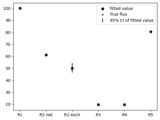
We see that INCAWrapper and INCA was able to obtain unbiased estimates of the true fluxes using INST 13C-MFA. The R2 exchange flux still has some uncertainty, but it is common for exchange fluxes not to be well determined [3]. Lets also inspect the numerical values of the fitted and true fluxes.
[19]:
fitted_and_true_fluxes = (
    estimated_fluxes
    .merge(true_fluxes, left_on="id", right_on="rxn_id")
    .rename(columns={"val": "fitted_flux", "flux": "true_flux"})
)
fitted_and_true_fluxes[['type', 'id', 'eqn', 'true_flux', 'fitted_flux', 'std', 'lb', 'ub']].round(3)
[19]:
| type | id | eqn | true_flux | fitted_flux | std | lb | ub | |
|---|---|---|---|---|---|---|---|---|
| 0 | Net flux | R1 | A -> B | 100.000 | 99.992 | 0.190 | 99.51167 | 100.479345 |
| 1 | Net flux | R2 net | B <-> D | 61.132 | 61.151 | 0.299 | 60.342355 | 61.896734 |
| 2 | Exch flux | R2 exch | B <-> D | 49.806 | 49.849 | 1.736 | 46.264288 | 54.217439 |
| 3 | Net flux | R3 | B -> C + E | 19.434 | 19.421 | 0.189 | 18.938698 | 19.950753 |
| 4 | Net flux | R4 | B + C -> D + E + E | 19.434 | 19.421 | 0.189 | 18.938698 | 19.950753 |
| 5 | Net flux | R5 | D -> F | 80.566 | 80.571 | 0.164 | 80.16627 | 80.97421 |
Again here we see that the incawrapper (and INCA) finds a good estimate of the true flux distribution.
9.2.1. References
[1] M. R. Antoniewicz, J. K. Kelleher, and G. Stephanopoulos, “Determination of confidence intervals of metabolic fluxes estimated from stable isotope measurements,” Metabolic Engineering, vol. 8, no. 4, pp. 324–337, Jul. 2006, doi: 10.1016/j.ymben.2006.01.004.
[2] M. R. Antoniewicz, J. K. Kelleher, and G. Stephanopoulos, “Elementary metabolite units (EMU): A novel framework for modeling isotopic distributions,” Metabolic Engineering, vol. 9, no. 1, pp. 68–86, Jan. 2007, doi: 10.1016/j.ymben.2006.09.001.
[3] W. Wiechert and K. Nöh, “Quantitative Metabolic Flux Analysis Based on Isotope Labeling,” in Metabolic Engineering, 1st ed., J. Nielsen, G. Stephanopoulos, and S. Y. Lee, Eds., Wiley, 2021, pp. 73–136. doi: 10.1002/9783527823468.ch3.